Computer Vision at Scale on SageMaker Jobs: Four Decisions

Training a vision model on millions of images is, more than anything, a data problem wearing an ML costume. The architecture can many times be the least interesting part. Everything around it is usually more fun: how we are getting images onto the GPU, running distributed training without hand-rolling process management, and wiring a chain of jobs together so that a failure nine hours into a run tells you exactly what broke instead of just turning red. Better yet, so you catch it before you burn the nine hours, with good logging and small test runs.

Amazon SageMaker jobs are a super solid way to build this kind of pipeline. Across a few recent projects, most recently a large-scale computer-vision pipeline, I have landed on four decisions that, in my opinion, mostly determine whether the build is linear and “boring” (the good kind) or a three-week debugging tour of CloudWatch (the ‘not-so-good’ kind):

Which SageMaker job primitive runs each step.
How image data reaches the GPU at scale.
How distributed training is launched and synchronized.
How each job’s boundaries are made explicit and operable.

One honest note before we dive in: only one of these four is really about computer vision. Decisions 1 and 4 are general SageMaker jobs hygiene that any big-data workload needs, and Decision 3 is general distributed training that images only make bite harder. Decision 2, the data layer, is where computer vision actually lives. I will flag each section as we go, because knowing which lessons are vision-specific and which are “any big job on SageMaker” is half of what makes them useful.

Who this is for#

This is written for ML and MLOps engineers who have trained models before and now have to do it at scale on AWS. You will get the most from it with at least some computer-vision experience: enough that a DataLoader, an augmentation pipeline, and an epoch are old friends, because I lean on those without re-explaining them. You do not need to be a SageMaker expert, since I introduce the pieces as they come up. And if you have so far only trained on datasets that fit on your laptop, you are exactly the person the scale gotchas here will save a week.

This is not an AWS tutorial, and we are not getting into SDK code! Check the ‘further reading’ section for that, or point your favorite LLM at the docs to wire up the exact calls. This is the set of things that actually bite, or that at least have bitten me before. So, let’s go!

Why big-data Computer Vision is mostly an I/O problem#

Before anything, a quick note: if you have only trained on datasets that fit on a local disk, the instinct is to worry about GPU memory and FLOPs. At a million images, with distributed training and a good enough budget, those are rarely the constraint. I/O is. Every epoch, each image has to travel from storage, through preprocessing and augmentation, into a batch, and onto the GPU, fast enough that the GPU never waits. Pull each one from object storage on demand and you are making millions of tiny requests per epoch while your expensive GPU sits idle on the network. So the first metric to watch is not always loss, it is GPU utilization. Under 80 percent means the data pipeline is your bottleneck, and more GPU will not help.

What makes this specifically a vision problem is the unit of data. A tabular row is a few hundred bytes and needs no decoding; an image is hundreds of kilobytes to several megabytes of compressed JPEG or PNG that has to be decoded, resized, and augmented before it is ever a tensor. That decode step alone is a real CPU cost, and it is the quiet reason the GPU starves. And one dial governs most of it: resolution. The pixels you train on set your batch size, your memory ceiling, your decode and augmentation cost, your storage footprint, and your accuracy, all at once. Pick it deliberately and early, because almost every number in the rest of this post moves with it.

Decision 1: pick the job primitive that matches the work#

Mostly general SageMaker. This is true for any big-data job, not just vision.

SageMaker is a family of job primitives, and two of them are the workhorses of a training pipeline. A Processing Job is the general-purpose worker: it runs a script, reads inputs from S3, writes outputs to S3, and disappears. It usually runs on CPU (though it can use GPU instances) and lacks the training toolkit and FSx mounting. Use it for data prep, preprocessing, evaluation, and metric aggregation. A Training Job is the GPU specialist: it carries SageMaker’s training toolkit, which launches distributed training cleanly, and it can mount an FSx for Lustre filesystem. Use it for training.

Three more are worth knowing even if you do not use them on a given project. A Batch Transform Job is the purpose-built primitive for bulk offline inference: it shards a dataset across instances and runs the forward pass with no inference loop to write, which is the managed alternative to scoring inside a Processing Job. A Hyperparameter Tuning Job wraps the training primitive to search a hyperparameter space across many runs. And an AutoML Job automates model building end to end, which is the wrong tool for a custom architecture but the right one for a quick standard baseline. Serving a model online is a separate world of endpoints (real-time, asynchronous, serverless), not jobs.

A pipeline is just a chain of those with S3 as the “bus” between steps: a CPU step turns your data source into a snapshot on S3, a GPU step trains and writes a checkpoint, a CPU step scores the held-out set.

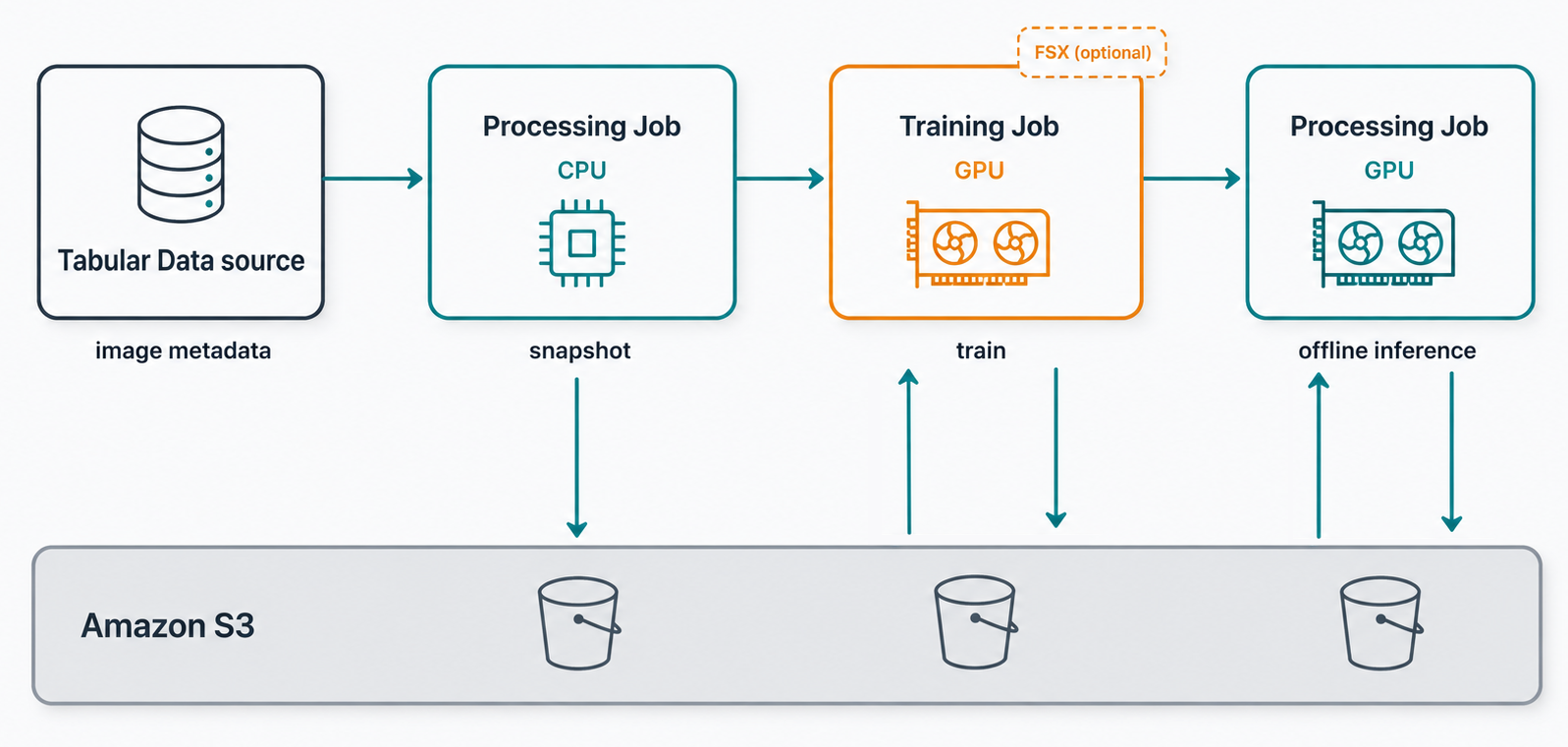
A generic SageMaker pipeline for training a computer-vision foundation model and running offline inference, built entirely from jobs and steps. Each step is a self-contained job that reads from and writes to S3.

The trap is reaching for one job type out of habit. I once ran an evaluation pass as a Training Job purely so it could mount FSx like the training step did, on the theory that consistency was tidy. It was not tidy, just wasteful: a CPU-only job paying for GPU plumbing it never touched. Match the primitive to the workload, not to the step before it. One pipeline habit worth building early: write each step’s output under the pipeline execution ID, so two runs at once cannot overwrite each other’s artifacts in S3.

Decision 2: design the data layer like it is the main event#

The computer-vision core of this post. If you skim one section, make it this one.

“We’ll cache the images” is not a design. There are real strategies with real tradeoffs, and the right one depends on dataset size and how often you re-run on the same data.

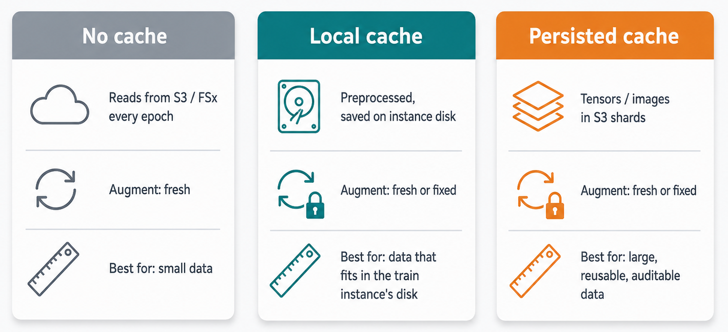
No cache. Read and preprocess from S3 (or FSx) on every access. Simple, fine for small datasets and debugging, brutal at scale because you pay the full I/O and preprocessing cost every epoch. Generally not the right call for the kind of problem we are dealing with here, though depending on how heavy your preprocessing is, it can be acceptable.
Local cache. Preprocess each image once, write it to instance disk, and read from disk after that. You can also choose to apply augmentations fresh per epoch so you do not freeze one augmentation outcome into the cache. Two details save you grief: key the cache on the full image path plus the target resolution, not the bare filename (or two files both called 001.png collide), and write through a temporary file and an atomic rename so a crash cannot leave a half-written file the next run trusts.
Persisted preprocessed cache. My favorite for most projects! Run it as a preprocessing job once, write the results to S3 in large tensor shards or actual image files, and fingerprint the preprocessing config so that a re-run with the same config skips the work entirely. This is the one for large datasets you train on repeatedly.

*The main caching strategies for large-scale computer-vision jobs, and the tradeoffs that decide between them.*

It helps to separate two things that often get muddled here: how your samples are laid out in storage, and how the bytes reach the training box. They are independent choices, and they stack.

Start with layout, and specifically sharding. Object storage charges a fixed overhead on every GET, so reading a million images as a million separate objects means a million tiny, latency-bound requests with the GPU idle in between. Sharding packs many samples into a handful of large container files, say a few thousand images per shard and a few hundred shards instead of a million objects, which turns those small random reads into a few big sequential ones that stream and parallelize cleanly across workers. This is exactly what the persisted cache above is doing when it writes large tensor shards. You can hand-roll that, which is what we did on that recent vision project, where the preprocessing was custom enough that a plain tensor dump was simplest, or you can reach for WebDataset, FFCV, or MosaicML Streaming, which give you the shard format and a tuned reader and shuffle buffer off the shelf. Same idea either way, the only question is whether you want to own the reader.

The second axis is transport. On SageMaker, Fast File mode streams objects from S3 with filesystem semantics and no upfront download, and it is the lightest thing to try first. FSx for Lustre is the step up: a POSIX filesystem backed by S3 that serves reads at local-disk speed once it is warm. My favorite setup stacks the two ideas, persisted sharded tensors living on an FSx volume, so you get the cheap sequential reads of sharding and the low latency of a local mount. Once you are on FSx there is little reason to also keep a separate local cache, since the mount loads about as fast. Whichever transport you pick, make FSx fail loud: if the mount is configured but unreachable, raise immediately rather than silently falling back to S3, because silent fallback gives you a job that trains at a tenth of the throughput you are paying for with nothing in the logs to tell you. And if it turns out that JPEG decode, not transport, is what is starving your GPU, push decoding and augmentation onto the GPU with a library like NVIDIA DALI.

Two knobs inside the data layer are pure computer vision, and worth setting on purpose rather than by accident. The first is what you persist. Re-encoded images (JPEG, PNG) are small and cheap to move but pay the decode cost on every read, and lossy JPEG re-compression can quietly degrade what the model sees, decoded tensors skip the decode but are much larger on disk and across the wire. The second is where augmentation sits. Cache after augmentation and every epoch sees the same frozen crops and color jitter, which throws away the regularization you wanted; cache the preprocessed-but-not-yet-augmented image instead and apply augmentation fresh at read time. For anything that leans on augmentation diversity, which is most vision training, persist before augmentation.

Decision 3: let the platform run distributed training#

General distributed training, not vision-specific, but image batches make it bite sooner.

The biggest mechanical change when you go multi-GPU on SageMaker is who owns the processes. Do not call torch.multiprocessing.spawn and set the master address yourself. Enable the distributed strategy on the training job and let the Deep Learning Container launch your script through torchrun. Your script becomes an ordinary single-process entry point that reads RANK, LOCAL_RANK, and WORLD_SIZE from the environment, and you never set the master address. torchrun sets it, and overriding it is a popular way to make a job hang forever.

A few rules keep distributed training honest: use LOCAL_RANK, not the global rank, for device placement; scope all side effects (checkpoint writes, logging, progress) to rank 0; aggregate loss weighted by each rank’s sample count rather than as a mean of means; and give process-group initialization a generous timeout so a slow cache build does not look like a dead rank.

Then there is the SageMaker special. Your first run will probably die on the first batch with “No space left on device,” which is baffling on an instance with terabytes of disk. The culprit is the 64 MB /dev/shm partition that SageMaker containers ship with, which PyTorch’s default DataLoader uses to pass tensors between workers. Vision hits this wall fast, because those tensors are decoded image batches, and a single batch at training resolution is easily tens to hundreds of megabytes. The fix can be a one-liner, set at import time:

import torch.multiprocessing
torch.multiprocessing.set_sharing_strategy("file_system")

That routes tensor IPC through the filesystem instead of /dev/shm shared memory, which can cost you throughput if that filesystem is slow. A few ways to keep it cheap:

Put the temp directory on fast local storage. The strategy writes to your temp dir, so point TMPDIR at instance-store NVMe (or a tmpfs, if you have the RAM to spare) rather than network-backed EBS, and “going through disk” stops being slow.
Move less data across the worker boundary. The IPC cost scales with how much each worker hands back, so decode and augment on the GPU (DALI, Kornia) or return compact uint8 tensors and convert on device, and there is simply less to ship.
Reuse workers. Set persistent_workers=True with a sane num_workers so you are not paying worker startup every epoch.

If you control the container you can size /dev/shm up and keep the default strategy instead; on managed SageMaker jobs you usually cannot, which is why the one-liner is the pragmatic fix.

Two more things I would assume in any serious run but that are easy to leave out: mixed precision (use bf16 on modern GPUs for roughly double the memory headroom and throughput) and the fact that plain DDP only works while the model fits on one GPU. When it does not, you move to FSDP or DeepSpeed ZeRO, which shard the model across GPUs.

Decision 4: make every job boundary explicit#

General MLOps hygiene, not vision-specific, included because at vision scale skipping it hurts most.

A framework that passes data between steps implicitly is really cool right up until something breaks, at which point the implicitness is exactly what hides the cause. SageMaker jobs force you to spell out every boundary, and you should lean into that. Make each step a standalone script with a clear contract: command-line arguments for its config and input paths, environment variables for infrastructure, and a defined S3 location for output. No shared in-memory state, no magic serialization. You can run any step by hand with the same arguments the pipeline would pass it.

Identity is part of that contract. Key everything off a job name you set when the run starts, and build the checkpoint path from it, so downstream steps reconstruct the path by string-building rather than querying a metadata service. (Watch for reserved names. SageMaker sets its own TRAINING_JOB_NAME inside training containers, so give yours a prefix.) Emit structured JSON logs tagged with that job name so your logs are queryable instead of a wall of text, and connect experiment tracking through an explicit endpoint rather than letting the orchestrator inject it for you.

The bonus: making every boundary explicit, and then running real data through at scale, tends to surface latent bugs that implicit wiring kept hidden for years. Explicit boundaries are not just operational hygiene, they are a debugging tool.

Finally, my summary list of problems that may bite you!#

A quick list to scan before you start, most of which are not in most tutorial:

First batch dies with a disk-space error. The 64 MB /dev/shm limit. Move DataLoader tensor IPC off it with the file-system sharing strategy (Decision 3), backed by fast local storage.
A custom environment variable gets silently overwritten. SageMaker reserves some names. Prefix yours.
A downstream step cannot find the checkpoint. The path depended on something non-deterministic. Build it from a name you set up front.
Distributed training launches and hangs. Usually a base image without the SageMaker training toolkit, so torchrun never launches. Use the AWS Deep Learning Container.
A corrupt image halts a multi-day run. At a million images it will happen. A bounded skip in the loader is a backstop; a cheap validation pass before training is the real answer.
GPU utilization sits at half. Not a crash, just money on fire, and it sends you back to the data layer.

Where your situation will differ#

This post mostly went into classification-style training on fixed-size images, scored offline. A few axes move the details, and the most common task types each have particularities worth a sentence:

Classification is the easy case: a tiny scalar or one-hot label that caches for free, evaluated with accuracy or AUC.
Object detection, which is most of my own background, attaches a variable number of boxes to each image, so targets are variable-length and you need a custom collate function. It is evaluated with mAP and IoU, and inference adds non-maximum suppression and usually wants a GPU, which flips the fixed-shape cache and CPU-inference choices above.
Semantic and instance segmentation carry full-resolution mask targets, so augmentation has to be applied identically to image and mask, the cache roughly doubles in size, and large images force tiling.
Generative models (diffusion, GANs) lean on latent caching (encode each image once, then train on the latents, the same idea as the persisted cache), use aspect-ratio bucketing to batch mixed sizes, and are judged by FID or CLIP score rather than accuracy.

Two more axes, briefly. Your images: gigapixel scans or satellite tiles cannot go into a batch whole, so you tile them and sample patches, and non-RGB or high-bit-depth data changes normalization and storage. Your serving mode: offline batch scoring is one world; real-time, asynchronous (great for large payloads like video), and serverless endpoints are another, and the latency you ship usually comes from inference-time optimization like ONNX, TensorRT, or quantization rather than from the training recipe. And before any of this, split your data so that no group leaks across train and test (all images from the same source or subject in one split) and de-duplicate near-identical images first, or your metrics will look better than your model actually is.

Closing#

A million images is an infrastructure problem with four moving parts: the job primitive per step, the data layer, how distributed training is launched, and how explicit your job boundaries are. Get those right and the model training itself becomes the easy, almost boring part, which is exactly where you want it.